Part 1: Reads to reference genome and gene predictions
1. Introduction
Cheap sequencing has created the opportunity to perform molecular-genetic analyses on almost anything. Traditional genetic model organisms benefit from years of efforts by expert genome assemblers, gene predictors, and curators. They have created most of the prerequisites for genomic analyses. In contrast, genomic resources are much more limited for those working on “emerging” model organisms or other species. These new organisms include most crops, animals and plant pest species, many pathogens, and major models for ecology & evolution.
The steps below are meant to provide some ideas that can help obtaining a reference genome and a reference geneset of sufficient quality for many analyses. They are based on (and updated from) work we did for the fire ant genome[1].
The dataset you will use represents ~0.5% of the fire ant genome. This enables us to perform a toy/sandbox version of all analyses within a much shorter time than would normally be required. For real projects, much more sophisticated approaches are needed! You can ask about these in the forum, or in person.
During this series of practicals, we will:
- inspect and clean short (Illumina) reads,
- perform genome assembly,
- assess the quality of the genome assembly using simple statistics,
- predict protein-coding genes,
- assess quality of gene predictions,
- assess quality of the entire process using a biologically meaningful measure.
Note: Please do not jump ahead. You will gain the most by following through each section of the practical one by one. If you’re fast, dig deeper into particular aspects. Dozens of approaches and tools exist for each step - try to understand their tradeoffs.
2. Software and environment setup
Test that the necessary bioinformatics software is available
Run seqtk. If this prints command not found, ask for help. Otherwise, move
to the next section. If that one is available and you see it’s help screen, we’ll suppose that everything else is too.
Set up directory hierarchy to work in
Start by creating a directory to work in. Drawing on ideas from Noble (2009)[2] and others, we recommend following a specific directory convention for all your projects. The details of the convention that we will use in this practical can be found here.
For the purpose of these practicals we will use a slightly simplified version of the directory structure explained above.
For each practical, you will have to create the following directory structure:
- main directory in your home directory in the format
(
YYYY-MM-DD-name_of_the_practical, whereYYYYis the current year,MMis the current month, andDDis the current day, andname_of_the_practicalmatches the practical). For instance, on the 24th of September 2024, you should create the directory2024-09-24_read_cleaningfor this practical. In the tutorial we will use this example directory name. - Inside this directory, create other three directories, called
input,tmp, andresults. - The directory
inputwill contain the FASTQ files. - The directory
tmpwill represent your working directory. - The directory
resultswill contain a copy of the final results.
Each directory in which you have done something should include a WHATIDID.txt
file in which you log your commands.
Being disciplined about structuring analyses is extremely important. It is similar to having a laboratory notebook. It will prevent you from becoming overwhelmed by having too many files, or not remembering what you did where.
Your directory structure should look like this (run tree in your home
directory):
2024-09-24-read_cleaning
├── input
├── tmp
├── results
└── WHATIDID.txt
Note: Once you create this directory structure, you can get this tree structure by running the
treecommand inside the directory ending with-read_cleaning.
3. Sequencing an appropriate sample
The properties of your data can affect the ability of bioinformatics algorithms to handle them. For instance, less diversity and complexity in a sample makes life easier: assembly algorithms really struggle when given similar sequences. So less heterozygosity and fewer repeats are easier.
Thus:
- A haploid is easier than a diploid (those of us working on haplo-diploid Hymenoptera have it easy because male ants are haploid).
- It goes without saying that a diploid is easier than a tetraploid!
- An inbred line or strain is easier than a wild-type.
- A more compact genome (with less repetitive DNA) is easier than one full of repeats - sorry, grasshopper & Fritillaria researchers! ;)
Many considerations go into the appropriate experimental design and sequencing strategy. We will not formally cover those here & instead jump right into our data.
4. Illumina short-read cleaning
In this practical, we will work with paired ends short read sequences from an Illumina machine. Each piece of DNA was thus sequenced once from the 5’ and once from the 3’ end. Thus, we expect to have two files per sequence.
However, sequencers aren’t perfect. Several problems may affect the quality of the reads. You can find some examples here and here.
Also, as you may already know, “garbage in – garbage out”, which means that reads should be cleaned before performing any analysis.
Setup and initial inspection using FastQC
Lets move to the main directory for this practical, so that everything we need and do and create is in one place:
# Remember that yours may have a different date, now or in future, so be careful to check if you copy-paste code
cd ~/2024-09-24-read_cleaning
After, create a symbolic link (or symlink) using ln -s from the reads files to the
input directory:
# Change directory to input
cd input

# Link the two compressed FASTQ files (remember that each correspond to one of
# the pair)
ln -s /shared/data/reads.pe1.fastq.gz .
ln -s /shared/data/reads.pe2.fastq.gz .

# Return to the main directory
cd ..
The structure of your directory should look like this (use the command tree):
2024-09-24-read_cleaning
├── input
│   ├── reads.pe1.fastq.gz -> /shared/data/reads.pe1.fastq.gz
│   └── reads.pe2.fastq.gz -> /shared/data/reads.pe2.fastq.gz
├── tmp
├── results
└── WHATIDID.txt
Now, you can start evaluating the quality of the reads reads.pe1.fastq.gz and
reads.pe2.fastq.gz. To do so, we will use
FastQC
(documentation).
FASTQC is a software tool to help visualise the characteristics of a sequencing run.
It can thus inform your read cleaning strategy.
Run FastQC on the reads.pe1.fastq.gz and reads.pe2.fastq.gz files.
The command is given below, where instead of YOUR_OUTDIR, you will need
replace YOUR_OUTDIR with the path to your tmp directory (e.g. if you main
directory is 2024-09-24-read_cleaning, you need to replace YOUR_OUTDIR with
tmp):
fastqc --nogroup --outdir YOUR_OUTDIR input/reads.pe1.fastq.gz
fastqc --nogroup --outdir YOUR_OUTDIR input/reads.pe2.fastq.gz
The --nogroup option ensures that bases are not grouped together in many of
the plots generated by FastQC. This makes it easier to interpret the output in
many cases. The --outdir option is there to help you clearly separate input
and output files. To learn more about these options run fastqc --help in the
terminal.
Note: Remember to log the commands you used in the
WHATIDID.txtfile.
Take a moment to verify your directory structure. You can do so using the tree
command (be aware of your current working directory using the command pwd):
tree ~/2024-09-24-read_cleaning
Your resulting directory structure
(~/2024-09-24-read_cleaning), should look like this:
2024-09-24-read_cleaning
├── input
│   ├── reads.pe1.fastq.gz -> /shared/data/reads.pe1.fastq.gz
│   └── reads.pe2.fastq.gz -> /shared/data/reads.pe2.fastq.gz
├── tmp
│   ├── reads.pe1_fastqc.html
│   ├── reads.pe1_fastqc.zip
│   ├── reads.pe2_fastqc.html
│   └── reads.pe2_fastqc.zip
├── results
└── WHATIDID.txt
If your directory and file structure looks different, ask for some help.
Now inspect the FastQC report. First, copy the files reads.pe1_fastqc.html and
reads.pe2_fastqc.html to the directory ~/www/tmp. Then, open the browser and
go to your personal module page (e.g., if your QMUL username is bob, the
URL will be https://bob.genomicscourse.com) and click on the ~/www/tmp link. After
that, click on one of the links corresponding to the reports files.
Question: What does the FastQC report tell you? If in doubt, check the documentation here and what the quality scores mean here.
For comparison, have a look at some plots from other sequencing libraries: e.g, [1], [2], [3]. NOTE: the results for your sequences may look different.
![[1]](/genomicscourse/current-year/practicals/reference_genome/img-qc/per_base_quality.png)
![[2]](/genomicscourse/current-year/practicals/reference_genome/img-qc/qc_factq_tile_sequence_quality.png)
![[3]](/genomicscourse/current-year/practicals/reference_genome/img-qc/per_base_sequence_content.png)
Clearly, some sequences have very low quality bases towards the end. Why do you think that may be? Furthermore, many more sequences start with the nucleotide A rather than T. Is this what you would expect?
Question:
- Which FastQC plots shows the relationship between base quality and position in the sequence? What else does this plot tell you about nucleotide composition towards the end of the sequences?
- Should you maybe trim the sequences to remove low-quality ends? What else might you want to do?
In the following sections, we will perform two cleaning steps:
- Trimming the ends of sequence reads using cutadapt.
- K-mer filtering using kmc3.
- Removing sequences that are of low quality or too short using cutadapt.
Other tools, including fastx_toolkit, BBTools, and Trimmomatic can also be useful, but we won’t use them now.
Read trimming
To clean the FASTQ sequences, we will use a software tool called cutadapt. As stated on the official website:
Cutadapt finds and removes adapter sequences, primers, poly-A tails and other types of unwanted sequence from your high-throughput sequencing reads.
Specifically, we will use cutadapt to trim the sequences.
Question: What is the meaning of
cutadaptoptions--cutand--quality-cutoff? (Hint: you can read a short description of the options by calling the commandcutadapt -h)
To identify relevant quality cutoffs, it is necessary to be familiar with base quality scores and examine the per-base quality score in your FastQC report.
We will run cutadapt with two options, --cut and/or --quality-cutoff,
corresponding to the number of nucleotides to trim from the beginning (--cut)
and end (--quality-cutoff) of the sequences.
Note: If you trim too much of your sequence (i.e., too large values for
--cutand--quality-cutoff), you increase the likelihood of eliminating important information. Additionally, if the trimming is too aggressive, some sequences may be discarded completely, which will cause problems in the subsequent steps of the pre-processing. For this example, we suggest to keep--cutbelow 5 and--quality-cutoffbelow 10.
The command to run cutadapt on the two reads files is reported below, where
BEGINNING and CUTOFF are the the two integer values corresponding to the
number of bases to trim from the beginning of the sequence and the quality
threshold (see the above note for suggestion about the values to use). Remember
that each .fq file can have a different set of values.
cutadapt --cut BEGINNING --quality-cutoff CUTOFF input/reads.pe1.fastq.gz > tmp/reads.pe1.trimmed.fq

cutadapt --cut BEGINNING --quality-cutoff CUTOFF input/reads.pe2.fastq.gz > tmp/reads.pe2.trimmed.fq
5. K-mer filtering, removal of short sequences
Let’s suppose that you have sequenced your sample at 45x genome coverage. This
means that every nucleotide of the genome was sequenced 45 times on average.
So, for a genome of 100,000,000 nucleotides, you expect to have about 4,500,000,000
nucleotides of raw sequence. But that coverage will not be homogeneous.
Instead, the real coverage distribution will be influenced by factors including DNA quality,
library preparation type, how was DNA packaged within the chromosomes (e.g., hetero vs. euchromatin)
and local GC content. But you might expect most of the genome to be covered between
20 and 70x.
In practice, this distribution can be very strange. One way of rapidly examining the coverage distribution before you have a reference genome is to chop your raw sequence reads into short “k-mers” of k nucleotides long, and estimate the frequency of occurrence of all k-mers. An example plot of k-mer frequencies from a haploid sample sequenced at ~45x coverage is shown below:
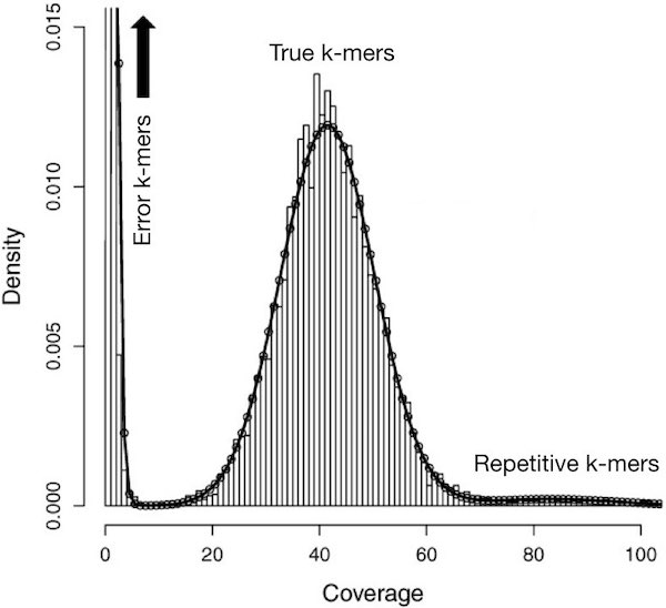
In the above plot, the y axis represents the proportion of k-mers in the dataset that are observed x times (called Coverage). As, expected, we observe a peak in the region close to 45, which corresponds to the targeted coverage.
However, we also see that a large fraction of sequences have a very low coverage (they are found only 10 times or less).
These rare k-mers are likely to be errors that appeared during library preparation or sequencing, or could be rare somatic mutations. Analogously (although not shown in the above plot) other k-mers may exist at very large coverage (up to 10,000). These could be viruses or other pathogens, or highly repetitive parts of the genome, such as transposable elements or simple repeats.
Note: Extremely rare and extremely frequent sequences can both confuse assembly algorithms. Eliminating them can reduce subsequent memory, disk space and CPU requirements considerably, making overall computing more efficient and friendly.
Below, we use kmc3 to “mask” extremely rare k-mers (i.e., convert each base in the sequences corresponding to rare k-mers into N). In this way, we will ignore these bases (those called N) because they are not really present in the species. Multiple alternative approaches for k-mer filtering exist (e.g., using khmer).
Here, we use kmc3 to estimate the coverage of k-mers with a size of 21 nucleotides. When the masked k-mers are located at the end of the reads, we trim them in a subsequent step using cutadapt. If the masked k-mers are in the middle of the reads, we leave them just masked. Trimming reads (either masked k-mers or low quality ends in the previous step) can cause some reads to become too short to be informative. We remove such reads in the same step using cutadapt. Finally, discarding reads (because they are too short) can cause the corresponding read of the pair to become “unpaired”. While it is possible to capture and use unpaired reads, we skip that here for simplicity. Understanding the exact commands – which are a bit convoluted – is unnecessary. However, it is important to understand the concept of k-mer filtering and the reasoning behind each step.
# To mask rare k-mers we will first build a k-mer database that includes counts
# for each k-mer.
# For this, we first make a list of files to input to KMC.
ls tmp/reads.pe1.trimmed.fq tmp/reads.pe2.trimmed.fq > tmp/file_list_for_kmc

# Build a k-mer database using k-mer size of 21 nucleotides (-k). This will
# produce two files in your tmp/ directory: 21-mers.kmc_pre and 21-mers.kmc_suf.
# The last argument (tmp) tells kmc where to put intermediate files during
# computation; these are automatically deleted afterwards. The -m option tells
# KMC to use only 4 GB of RAM.
kmc -m4 -k21 @tmp/file_list_for_kmc tmp/21-mers tmp

# Mask k-mers (-hm) observed less than two times (-ci) in the database
# (tmp/21-mers). The -t option tells KMC to run in single-threaded mode: this is
# required to preserve the order of the reads in the file. filter is a
# sub-command of kmc_tools that has options to mask, trim, or discard reads
# contain extremely rare k-mers.
# NOTE: kmc_tools command may take a few seconds to complete and does not
# provide any visual feedback during the process.
kmc_tools -t1 filter -hm tmp/21-mers tmp/reads.pe1.trimmed.fq -ci2 tmp/reads.pe1.trimmed.norare.fq
kmc_tools -t1 filter -hm tmp/21-mers tmp/reads.pe2.trimmed.fq -ci2 tmp/reads.pe2.trimmed.norare.fq

# Check if unpaired reads are present in the files
cutadapt -o /dev/null -p /dev/null tmp/reads.pe1.trimmed.norare.fq tmp/reads.pe2.trimmed.norare.fq

# Trim 'N's from the ends of the reads, then discard reads shorter than 21 bp,
# and save remaining reads to the paths specified by -o and -p options.
# The -p option ensures that only paired reads are saved (an error is raised
# if unpaired reads are found).
cutadapt --trim-n --minimum-length 21 -o tmp/reads.pe1.clean.fq -p tmp/reads.pe2.clean.fq tmp/reads.pe1.trimmed.norare.fq tmp/reads.pe2.trimmed.norare.fq

# Finally, we can copy over the cleaned reads to results directory for further analysis
cp tmp/reads.pe1.clean.fq tmp/reads.pe2.clean.fq results
Inspecting quality of cleaned reads
Which percentage of reads have we removed overall? (hint: wc -l can count
lines in a non-gzipped file). Is there a general rule about how much we should
be removing?
6. References
-
Wurm, Y., Wang, J., Riba-Grognuz, O., Corona, M., Nygaard, S., Hunt, B.G., Ingram, K.K., Falquet, L., Nipitwattanaphon, M., Gotzek, D. and Dijkstra, M.B., 2011. The genome of the fire ant Solenopsis invicta. Proceedings of the 2012. National Academy of Sciences, 108(14), pp.5679-5684.
-
Noble, W.S., 2009. A quick guide to organizing computational biology projects. PLoS computational biology, 5(7), p.e1000424.
7. Further reading
-
MARTIN Marcel. Cutadapt removes adapter sequences from high-throughput sequencing reads. EMBnet.journal, [S.l.], v. 17, n. 1, p. pp. 10-12, may 2011. ISSN 2226-6089. doi: https://doi.org/10.14806/ej.17.1.200.
-
Kokot, M., Długosz, M. and Deorowicz, S., 2017. KMC 3: counting and manipulating k-mer statistics. Bioinformatics, 33(17), pp.2759-2761.
8. Bonus questions if you’re done early
- Which read cleaners exist and are the most popular today? Which would you use for Illumina data? And for long-read data? Why?
- How do read cleaning strategies for RNAseq and DNAseq differ?
- Can having an existing genome assembly help with read cleaning? How?